Statistical Inference
Last updated: Sep 26, 2025Table of Contents
- Introduction
- Parameter Estimation
- Hypothesis Testing
- Normality Tests
- Types of Hypothesis Tests
- One-Way ANOVA Test
- Multi-way ANOVA
- Non-Parametric Hypothesis Testing
Introduction
In statistical inference, a parameter is a fixed, unknown numerical value that describes a characteristic of an entire population. You can study the characteristics/estimators (eg. mean, SD, proportion, etc.) of the parameter on a sample of the population. You can do parameter estimation.
Parameter Estimation
It can be point estimation or interval estimation. A point estimate is a single numerical value that serves as the “best guess” or single-point approximation of an unknown population parameter. While interval estimation provides a range of values with a certain level of confidence. Confidence interval is a range of values that is likely to contain the true population parameter with a certain level of confidence. You can study the distribution of the estimate of that parameter using statistical methods.
Hypothesis Testing
Unlike Estimation, in Hypothesis testing on a parameter, we have a pre-idea of the population parameter (which you may arrive at with some EDA). Hypothesis testing is a method of testing that claim or hypothesis about a population parameter using sample data. It involves setting up a null hypothesis (H0) and an alternative hypothesis (H1), and then using statistical methods to determine whether the null hypothesis can be rejected in favor of the alternative hypothesis. H1 can be omitted if you you’re qualitatively sure about H0 and just want to quantitatively test it.
In hypothesis testing, you often look for a single numeric value called test statistic and if it lies in the region of acceptance, then you accept H0, and if it lies in the critical region, you reject H0. If we incorrectly reject H0, it’s called a Type 1 error, and if we incorrectly accept H0, it’s called Type 2 error. It’s difficult to minimise both errors simultaneously, so we need to see which is practically more critical and then focus on minimizing that type of error.
We have 2 probabilities:
Alpha (α): Probability of Type 1 error; False positive rate
Beta (β): Probability of Type 2 error; False negative rate
Commonly, \(\alpha\) (called significance level) is set at 0.05 (5%), meaning a 5% risk of Type 1 error is tolerated in the test decision. \(\beta\) is often set between 0.10 and 0.20 (10% to 20%), reflecting the risk of Type 2 error. The lower the \(\beta\), the higher the power of the test (1−β).
Normality Tests
We’ll study this before moving to hypothesis tests like z-test and t-test. Normality tests check if the data follows a normal (Gaussian) distribution. This is important because many parametric tests, including z-test and t-test, assume normality.
A normality test’s null hypothesis \(H_0\) states that the data is normally distributed; rejecting it means data significantly deviates from normal.
1. Boxplot
- A boxplot is a simple graphical tool that displays the distribution of data through quartiles and highlights outliers.
- It helps visually assess symmetry and detect skewness or extreme values—signs the data may not be normal.
boxplot(x)
2. Q-Q Plot (Quantile-Quantile Plot)
- A Q-Q plot graphs the quantiles of the data against the quantiles of a normal distribution.
- You first use
qqnorm()to generate the basic Q-Q plot of your data. - Then, you use
qqline()to add the reference line to this plot. - You then look at the resulting plot: if the data points from
qqnorm()fall closely along theqqline(), it indicates that the data is approximately normally distributed. Deviations from the line suggest that the data does not follow a normal distribution
3. Shapiro-Wilk Test
- A statistical test specifically designed to test normality, especially effective for small to medium-sized samples (<2000).
- Null hypothesis: sample comes from a normal distribution.
- A p-value > 0.05 suggests the data is likely normal; p-value < 0.05 suggests non-normality.
- The W statistic measures how well your sample data fits a normal distribution, with values closer to 1 indicating better fit.
shapiro.test(your_data_vector)function in R is used for this purpose.
4. Kolmogorov- Smirnov Test
ks.test(x, "pnorm", mean=mean(x), sd=sd(x))
Here also the null hypothesis is that the sample is normally distributed. A p-value > 0.05 indicates acceptance of the null hypothesis. A D-value is also generated which represents the maximum distance between your sample’s cumulative distribution function (CDF) and the CDF of a perfect normal distribution. A larger D-value indicates a greater deviation from normality.
This test is used for larger datasets cf. Shapiro-Wilks.
5. Lilliefors (Kolmogorov-Smirnov) Test
This is a variant of the earlier K-S test and may give a slightly different p-value.
install.packages(nortest)
library(nortest)
lillie.test(your_data_vector)
To conclude :
- Use boxplots or Q-Q plots for a quick visual check of normality.
- Confirm with Shapiro-Wilk test for small/medium datasets, or K-S test for larger datasets.
- Interpret p-values:
- p>0.05 → Fail to reject normality (data may be normal)
- p<0.05 → Reject normality (non-normal data)
Parametric Hypothesis Tests
1. Z Test
A z test tests a hypothesis of population mean based on a sample mean. It is a type of hypothesis test which tests if the “actual” sample mean is significantly different from a “hypothesized” population mean. It’s a fun fact that even if the difference between these 2 means may be substantial, it may not be statistically significant if the region of acceptance is not breached !
In z-test, \(H_0\) = sample mean is statistically similar to population mean
and \(H_1\)= sample mean is statistically different (+ or -) from the population mean
Assumptions
The z-test assumes :
- Sample size is large (n > 30) or the population is normally distributed. For large sample size, normality is assured as per the Central Limit Theorem. When in doubt, you can use a normality test (e.g., Shapiro-Wilk) or a histogram to check this.
- Population standard deviation (σ) is known : You can assume a value if not known.
- Data is independent
Key Features
- The z-test statistic (\(z\)) is calculated as:
\(z = \frac{\overline{x}-\mu}{\sigma/\sqrt{n}}\)
where \(\overline{x}\) is the “actual” sample mean, \(\mu\) is the “hypothesized” population mean, \(\sigma\) is the “known/guessed” population standard deviation, and \(n\) is the sample size. The quantity \(({\sigma/\sqrt{n}})\) is also called standard error of the mean. - The result (z-score) tells how many standard deviations the sample mean is from the population mean.
Practical Steps
- State the null and alternative hypothesis.
- Choose the significance level (\(\alpha\)) and use it to find the critical value from the z-table.
- Calculate the z statistic using the formula for \(z\).
- Compare the statistic with the critical value to decide to accept or reject the null hypothesis.
- Alternatively, compare the p-value (tail area after \(z\)) with \(\alpha\) (tail area after critical value) to decide to accept (\(p\)>\(\alpha\)) or reject the null hypothesis
In essence, we are converting our chosen parameter into a \(z\) score having a standard-normal \(\mathcal{N}\)(0,1) distribution. Graphically, the distribution of \(z\) would be as follows :
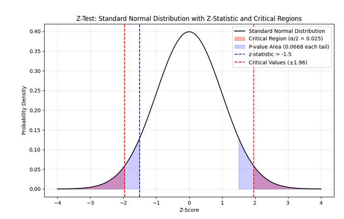
The midpoint \(z\)=0 denotes perfect compliance with the null hypothesis \(H_0\). The area other than critical region is the region of acceptance. Again note that z-test is mainly limited to testing a hypothesis of population mean based on a sample mean.
R function
In R, you can use the z.test() function from the BSDA package to perform z test on a single numeric column of a dataframe (i.e. one-sample z-test).
z.test(x, mu, sigma.x)
- x: Numeric vector of sample data.
- mu: Hypothesized population mean.
- sigma.x: Known population standard deviation.
Default: alternative = "two.sided", conf.level = 0.95.
2. T Test
Z-test is great for example in analyzing the mean gene expression across thousands of microarray measurements or say in aggregated read counts in whole-genome sequencing, where population standard deviation has been well-characterized in prior studies. But consider comparing the mean expression of a particular gene in two small groups of patients (say n = 15 per group) for a disease study. In such cases where population variance is unknown and/or sample size is small, t-test is preferred. Like z-test, normality of data is needed for t-test as well.
Like the z-test, the t-test allows you to transform your data into a score fitting a known distribution, but here the distribution is Student’s t. For smaller sample sizes (n < 30), the t-distribution is wider and has larger critical values than the standard normal (z) distribution. This means that the t-test requires stronger evidence (a larger absolute test statistic) to reject the null hypothesis. However the t-score tends to be smaller because its given by :
\(t = \frac{\overline{x} - \mu}{s / \sqrt{n}}\)
where \(s\) is the sample standard deviation and is usually larger than the population standard deviation \(\sigma\) used in z-test.
In R, you can use the built-in t.test() function to perform a t-test on a numeric column:
t.test(x, mu)
Apart from x and mu, some other parameters can be passed to the function, such as alternative to specify the alternative hypothesis, var.equal to specify whether the variances of the two groups are equal, paired to specify whether the data is paired or not and conf.level to specify the confidence level (eg. 0.95) of the confidence interval.
The output of the t.test() function is a dataframe with columns like output$statistic, output$conf.int,output$p.value, output$parameter(for degrees of freedom), etc.
Types of T Tests
-
One-sample t test :
Compares the mean of a single sample to a known population mean.
-
Two-sample t test:
Compares the means of two independent samples to see if they are significantly different.
-
Independent samples t test:
Compares the means of two independent samples to see if they are significantly different.
In the default pooled test version, we need to check the statistical similarity in the variances of the 2 samples using:var.test(data$sample1, data$sample2)But even if the variances are not equal, the test can still be used using the
var.equal=Falseargument (Welch’s t-test).
Eg.t.test(data$sample1, data$sample2, alternative="greater", paired = TRUE) -
Paired t test:
Similar to independent samples t test, but here both groups are the same sample under different conditions. Here you’ll use the
paired=Trueargument int.test().
Here it’s mandatory to first test the normality of the difference between the two samples.data$diff <- data$before_treat - data$after_treat shapiro.test(data$diff)Here
alternative = "greater"specifies that the alternative hypothesis is that the mean ofbefore_treatis greater than the mean ofafter_treat.
Note on two-sample t-tests : In these tests, by default we assume that the experimenter has no indication of a directional hypothesis (e.g., no prior evidence suggesting the values of sample-1 are greater than sample-2). Thus
alternative = "two.sided"argument is assumed by default. However if we have a directional research question like “Is the new drug better than the old one?”, then we can specifyalternative = "greater"oralternative = "less"depending on the direction of the hypothesis, and its called a one-tailed/one-sided test. -
3. One way ANOVA Test
Consider a dataset having 3 groups of data, each with a different mean. We want to test if the means of these groups are significantly different from each other.
This is an example of a multi-category dataset. When you perform multiple t-tests for many-category data instead of one ANOVA test, the probability of making a Type I error (false positive) increases due to the cumulative effect of multiple comparisons.
Here’s why:
- For each individual t-test, the significance level \(\alpha\) (e.g., 0.05) is the probability of falsely rejecting the null hypothesis (Type I error).
- If you perform, say, \(m\) independent t-tests, the probability of not making a Type I error in any one test is \(1 - \alpha\).
- The probability of not making any Type I errors in all \(m\) tests is \((1 - \alpha)^m\).
- Therefore, the probability of making at least one Type I error across all tests is:
- For example, with \(\alpha = 0.05\) and 6 tests (like 4 groups → 6 pairwise tests), this probability becomes:
which means a 26.5% chance of one or more false positives among the tests—much higher than the nominal 5%.
Why ANOVA helps
- ANOVA (Analysis of Variance) performs one overall test by comparing all groups simultaneously.
- The Type I error rate for this single test stays controlled at \(\alpha\) (e.g., 5%), avoiding inflation caused by multiple comparisons.
- If ANOVA is significant, you can then perform post hoc tests with corrections to identify specific group differences while controlling overall error.
Key Concepts and Hypotheses
-
Null Hypothesis (H0): All group means are equal.
\[H_0: \mu_1 = \mu_2 = \mu_3 = \dots = \mu_k\] -
Alternative Hypothesis (Ha): At least one group mean is different.
\(H_a: \text{At least one } \mu_i \ne \mu_j\) for some \(i \neq j\)
This means that if you reject \(H_0\), you conclude that not all groups have the same mean.
Assumptions for One-Way ANOVA
- Independence: Observations are independent within and across groups.
- Normality: The dependent variable is approximately normally distributed in each group.
- Homogeneity of Variance: The variances in each group are approximately equal.
You can check these with normality tests (Shapiro-Wilk), visualization (Q-Q plots), and variance tests (Levene’s test).
Core Idea: Partitioning Variance
ANOVA decomposes total variation in the data into two components:
- Between-Groups Variance (Variance due to group differences):
- How much the group means differ from the overall mean.
- Within-Groups Variance (Variance within each group):
- How much individual observations differ from their respective group means.
Calculations Step-by-Step
-
Calculate the Grand Mean (\(\bar{x}\)): The mean of all data points combined.
-
Calculate the Group Means (\(\bar{x}_i\)): The mean of each group \(i\), for \(i = 1, 2, \dots, k\).
-
Sum of Squares Between Groups (SSB):
\[SSB = \sum_{i=1}^k n_i (\bar{x}_i - \bar{x})^2\]where \(n_i\) is the number of observations in group \(i\).
-
Sum of Squares Within Groups (SSW):
\[SSW = \sum_{i=1}^k \sum_{j=1}^{n_i} (x_{ij} - \bar{x}_i)^2\] -
Total Sum of Squares (SST):
\[SST = \sum_{i=1}^k \sum_{j=1}^{n_i} (x_{ij} - \bar{x})^2 = SSB + SSW\] -
Degrees of Freedom:
- Between groups degrees of freedom: \(df_b = k - 1\)
- Within groups degrees of freedom: \(df_w = N - k\)
- Total degrees of freedom: \(df_t = N - 1\)
-
Mean Squares:
- Mean Square Between (MSB): \(MSB = \frac{SSB}{df_b}\)
- Mean Square Within (MSW): \(MSW = \frac{SSW}{df_w}\)
-
F-statistic:
\[F = \frac{MSB}{MSW}\]This ratio measures how large the variance between groups is compared to variance within groups. A large \(F\) suggests group means differ more than expected by chance.
Decision Rule
-
Compare the calculated \(F\)-statistic to the critical \(F\)-value from the \(F\)-distribution table at chosen significance level \(\alpha\) (usually 0.05) and degrees of freedom \((df_b, df_w)\).
-
Alternatively, compute the p-value for the observed \(F\).
-
If \(F_{calculated} > F_{critical}\) or \(p \leq \alpha\), reject \(H_0\) (means differ).
-
Otherwise, do not reject \(H_0\) (no evidence of differences).
Code example
# Load data
data <- read.csv("One way anova.csv")

# Check data
head(data)
# Expected columns: rhr (numeric), age.group (factor or character)

# Convert group variable to factor if needed
data$age.group <- as.factor(data$age.group)


# Subset data by group
gr_A <- subset(data, age.group == "A")$rhr
gr_B <- subset(data, age.group == "B")$rhr
gr_C <- subset(data, age.group == "C")$rhr


# Test normality of each group
shapiro.test(gr_A)
shapiro.test(gr_B)
shapiro.test(gr_C)

qqnorm(gr_A)
qqline(gr_A)

qqnorm(gr_B)
qqline(gr_B)

qqnorm(gr_C)
qqline(gr_C)

# Display statistical summary of each group
library(dplyr)
data %>%
  group_by(age.group) %>%
  summarise(
    count = n(),
    mean = mean(rhr, na.rm = TRUE),
    sd = sd(rhr, na.rm = TRUE)
  )

# Shortcut for normality test of all groups
library(dplyr)
data %>%
  group_by(age.group) %>%
  summarise(
   p_value = shapiro.test(rhr)$p.value
  )


# Leveny test to check the homogeneity of variance assumption in ANOVA
# Homogeneity of variance is assumed if p > 0.05
library(car)
leveneTest(rhr ~ age.group, data = data)


# Perform One-Way ANOVA: to test if the effect of age.group on rhr is statistically significant
anova_result <- aov(rhr ~ age.group, data = data)

# Summary of ANOVA test
summary(anova_result)
# F value may be > 1. Still, a p-value of greater than 0.05 confirms that F value is not statistically significant.
Multi-way ANOVA
If there is more than one column/group which influences the value column rhr, then we’ll run :
aov(rhr ~ gr1+gr2, data= data)
Note that if the dataset is in the form of a data frame or matrix, you’ll need to convert it to a pivot table before running the aov:
library(tidyverse)
long_df <- pivot_longer(rbd, cols = B1:B5, names_to = 'blocks', values_to = 'value')
This would convert this:
Variety,B1,B2,B3,B4,B5
A,20,26,30,28,23
B,6,12,10,9,7
C,12,15,16,14,14
D,17,10,20,23,20
E,28,26,23,33,30
F,70,62,56,64,75
to
Variety,blocks,value
A,B1,20
A,B2,26
A,B3,30
A,B4,28
A,B5,23
B,B1,6
B,B2,12
B,B3,10
B,B4,9
B,B5,7
C,B1,12
C,B2,15
C,B3,16
C,B4,14
C,B5,14
D,B1,17
D,B2,10
D,B3,20
D,B4,23
D,B5,20
E,B1,28
E,B2,26
E,B3,23
E,B4,33
E,B5,30
F,B1,70
F,B2,62
F,B3,56
F,B4,64
F,B5,75
which is suitable for running ANOVA.
4. Completely Randomized Design (CRD)
Non Parametric Hypothesis Testing
These are also called Distributin-free tests. They work on non-normal (often small data) data and in ALL cases of ordinal data. They generally require lesser assumptions.
1. Mann Whitney U-Test (Wilcoxon Rank-Sum Test)
This is an alternative to the Independent Sample T-Test.
\(H_0\) = Median of the 2 groups are similar
Given two independent samples, group 1 with size \(n_1\), and group 2 with size \(n_2\):
- Rank all values together (lowest gets rank 1, highest gets rank \(n_1 + n_2\)). If tied values, use average rank.
- Sum ranks for each group: Let \(R_1\) be the sum for group 1, \(R_2\) for group 2.
-
Calculate the U statistics:
\(U_1 = n_1 n_2 + \frac{n_1(n_1 + 1)}{2} - R_1\)
\(U_2 = n_1 n_2 + \frac{n_2(n_2 + 1)}{2} - R_2\) -
The final test statistic is \(U = \min(U_1, U_2)\).
- Compare \(U\) to critical values from table. If \(U\) \(\le\) \(U_{table}\), we reject \(H_0\) meaning that the 2 groups have stat. different medians.
R code:
To compare two independent groups, e.g., groups based on col1 with numeric outcomes in col2:
# Assuming df$col1 is grouping variable, df$col2 is numeric response
wilcox.test(col2 ~ col1, data = df, paired = FALSE)
If you want to compare two separate numeric vectors, for example df$col1 and df$col2 directly:
wilcox.test(df$col1, df$col2, paired = FALSE)
2. Wilcoxon Signed Test
This is an alternative to the parametric Paired T-Test.
Given paired data, for each pair:
- Calculate the difference for each pair: \(d_i = y_i - x_i\).
- Test statistic: \(W = \min(N_{+}, N_{-})\) where \(N_+\) is the no. of +ve differences and \(N_-\) is the no. of -ve differences.
- Decision: Compare \(W\) to table critical value (given \(n\) and α) or interpret p-value. Reject \(H_0\) if \(W\) is less than table value or p-value is below α.
3. Wilcoxon Signed Rank Test
The sign test can be made more robust when paired data differences can be meaningfully ranked by absolute magnitude. Adding some ranking logic, the process becomes:
Given paired data, for each pair:
- Calculate the difference for each pair: \(d_i = y_i - x_i\).
- Remove zero differences (\(d_i = 0\)) from consideration; let remaining pairs have \(n\) values.
- For all nonzero differences, take the absolute value and rank them (lowest to highest). Average ranks for ties.
- Assign ranks their original sign (+ for positive, − for negative differences).
- Sum positive ranks (\(T_{+}\)) and sum negative ranks (\(T_{-}\)).
- Test statistic: \(W = \min(T_{+}, T_{-})\) for small samples (\(n \leq 30\)).
- For large \(n\), use asymptotic normal approximation for \(Z\)-score or p-value.
- Decision: Compare \(W\) to table critical value (given \(n\) and α) or interpret p-value. Reject \(H_0\) if \(W\) is less than table value or p-value is below α.
R code :
To compare two independent groups, e.g., groups based on col1 with numeric outcomes in col2:
# Assuming df$col1 is grouping variable, df$col2 is numeric response
wilcox.test(col2 ~ col1, data = df, paired = TRUE)
If you want to compare two separate numeric vectors, for example df$col1 and df$col2 directly:
wilcox.test(df$col1, df$col2, paired = TRUE)
If you are certain of the direction of change, e.g. col2 having lesser values than col1, then you can specify \(H_1\) and do a one-sided test:
wilcox.test(df$col1, df$col2, paired=TRUE, alternative="greater")
4. Kruskal-Wallis (KW) Test
This is the alternative to the One-way ANOVA test for no. of studied groups (k) > 2 .
Given \(k\) independent groups with sample sizes \(n_1, n_2, ..., n_k\), total sample size \(N = \sum_{i=1}^k n_i\):
- Combine all data values from all groups and assign ranks \(R_{ij}\) (average ranks for ties) across the entire pooled data.
- Calculate the sum of ranks for each group:
- The Kruskal-Wallis test statistic \(H\) is computed as:
- For large samples, \(H\) approximately follows a chi-square distribution with \(k-1\) degrees of freedom.
- Decision rule: Reject the null hypothesis \(H_0\) (that all group medians are equal) if
or if the computed \(H\) exceeds the critical chi-square value for \(k-1\) degrees of freedom at significance level \(\alpha\).
R code:
For comparing more than two independent groups stored in col1 with numeric response col2:
kruskal.test(col2 ~ col1, data = df)